Generalized Jacobian inverses and Kinetic Energy Minimization
In my last post, I discussed how one may obtain a unique solution while inverting control Jacobians by constraining the generalized inverse’s null space to correspond to a velocity and acceleration null space. The way to do this was to show that the 
Here, I will discuss an alternative approach that produces the same result but works with the dual, which corresponds to velocity projections. The approach is to compute the Jacobian inverse using Lagrange multipliers in a way that minimizes Kinetic Energy in the entire control space, which includes the task’s null space.
If the previous paragraph sounded like jargon, please read my control tutorial and learn about Lagrange multipliers.
Let’s dive in by specifying our original equation and the Lagrangian with a generalized kinetic energy term:

A solution that extremizes the Lagrangian will have zero gradients with respect to both the generalized velocities and the lagrange multipliers:
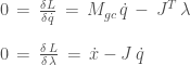
In order to resolve the Lagrange multiplier, we have to substitute 


Substituting this in our original equation, we have:

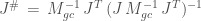
Which finally gives us

along with
You may double check that this is indeed the dynamically consistent generalized inverse that corresponds to the acceleration null space [1,2]. Deriving the dynamically consistent generalized inverse using Lagrange multipliers and the dual problem, help us state that it minimizes kinetic energy in the generalized coordinates. Or that this is the inertia regularized inverse. All three interpretations are correct.
References:
Generalized Jacobian inverses and acceleration null spaces
To start, if you are unfamiliar with robot control, consider reading this tutorial for a detailed introduction to the basic mathematics behind model based nonlinear robot control. The tutorial includes an introduction into whole-body control, and discusses how to perform motor tasks by projecting actuator forces through an articulated body’s nonlinear kinematics. For the post’s remainder, I will assume that you are already somewhat familiar with force control, and with potential issues with controlling task-redundant robots.
Let us first consider the task of controlling a force at a robot’s hand. We first present the kinematic Jacobian, which relates velocities and forces in task coordinates and the robot’s generalized coordinates.

Where x and (q, gc) are the task and generalized coordinates respectively. Using these identities, one may compute hand velocities when given joint velocities, and may compute joint (motor) torques given a desired force to be applied at the hand.
At times, however, one must invert the Jacobian, which is an underconstrained problem when robots have more degrees-of-freedom than the task at hand. Jacobian inverses are useful while performing multiple tasks if one wants to ensure that tasks don’t interfere with each other. One way to do this, presented in the tutorial and in a paper by Khatib (Khatib ’90), is to constrain the inverse by requiring its null space to be an acceleration null space. i.e., If

then the null space generalized forces 

Please note that unlike our notation, which uses indicative subscripts, Khatib’s notation uses different symbols for forces and inertias in different coordinates. So we have generalized inertias
, task space inertias
, generalized forces
etc.
The question then, is how one might compute this acceleration null space. Note that since the Jacobian relates velocities, a generic Moore-Penrose pseudoinverse‘s null space is already a velocity null space. Redundant robots, however, have infinitely many velocity null spaces corresponding to different generalized inverses, but only have a unique acceleration null space. This corresponds to the dynamically consistent generalized inverse given in Khatib’s paper:

If you did not understand how this was derived, please read the “Energy Equivalence and Operational Dynamics : Hand” section in Samir’s control tutorial.
Using this formulation, you can do cool stuff like pressing a doorbell with a robot’s hand while balancing a tray of cupcakes (yum!) on the robot’s elbow. An acceleration null space will guarantee that the elbow’s motions won’t interfere with the hand. Try it out!
References:
